Functions
Challenge 1: name_column()
Write a function called name_column that, given a data frame name and a number, will return the column name associated with that column number. Add an error message if the column number is < 1, or if the number exceeds the number of columns in the data frame. Test the function using the penguins data frame from the package palmerpenguins.
# For installing the package:
remotes::install_github("allisonhorst/palmerpenguins")
Challenge 2: Weight-Length relationship
The length-weight relationship for fish is \(W=aL^b\), where \(L\) is total fish length (cm), \(W\) is the expected fish weight (gr) and, \(a\) and \(b\) are species-dependent parameter values. In the table below, some examples from Peyton et al. (2016):
| sci_name | common_name | a_est | b_est |
|---|---|---|---|
| Chanos chanos | Milkfish | 0.0905 | 2.52 |
| Sphyraena barracuda | Great barracuda | 0.0181 | 3.27 |
| Caranx ignobilis | Giant trevally | 0.0353 | 3.05 |
-
Recreate the table above as a data frame stored as
fish_params. Then, write a function calledfish_weightthat allows a user to only enter the common name (argumentfish_name) and total length (argumenttot_length) (in cm) of a fish, to return the expected fish weight in gr. -
Test it out for different species and lengths. Add any error message you consider appropriate.
-
Now, try creating a vector of lengths (e.g., 0 to 100, by increments of 1) and ensuring that your function will calculate the fish weight over a range of lengths for the given species (try this for Great barracuda, storing the output weights as
greatbarra_weights.
Challenge 3: Monthly precipitation
We are interested in understanding the monthly variation in precipitation in Gainesville, FL. We’ll use some data from the NOAA National Climatic Data Center. Each row of the data file (gainesville-precip.csv) is a year (from 1961-2013) and each column is a month (January - December).
Write a function that:
- Imports the data.
- Calculates the average precipitation in each month across years.
- Plots the monthly averages as a simple line plot.
Don’t forget to document (describing what the function does) and test.
Challenge 4: Von Bertalanffy growth function
The Von Bertalanffy Growth Model (VBGM) describes the body growth in length of most fish, i.e.
\(L_t = L_{\infty} \left[ 1 - e^{-K(t-t_0)} \right]\) where \(L_t\) is the body length at age \(t\), \(L_{\infty}\) is the asymptotic or theoretical maximum length, \(K\) is the growth coefficient, and \(t_0\) is the theoretical age when length equals zero.
-
Write a function that returns the length given a specific age and a set of parameters
\((L_{\infty}, K, t_0)\) -
Next we will be working with biological data for Black Drum from Virginia waters of the Atlantic Ocean (view, download, meta-data). Download the data and save it as a .csv with the name
BlackDrum2001.csv. The data should look like:
library(tidyverse)
library(kableExtra)
blackdrum <- read.csv("https://raw.githubusercontent.com/droglenc/FSAdata/master/data-raw/BlackDrum2001.csv")
head(blackdrum)
## # A tibble: 6 x 9
##    year  agid spname     month   day weight    tl sex     otoage
##   <int> <int> <chr>      <int> <int>  <dbl> <dbl> <chr>    <int>
## 1  2001     1 Black Drum     4    30   15.7  788. male         6
## 2  2001     2 Black Drum     5     2   12.4  700  male         5
## 3  2001     3 Black Drum     5     3   74   1295  female      61
## 4  2001     4 Black Drum     5     3   47   1035  female      15
## 5  2001     5 Black Drum     5    10   NA   1205  unknown     33
## 6  2001     6 Black Drum     5    10   NA   1155  female      19
The VBGM, as well as most other growth models, is a non-linear model that requires non-linear statistical methods to estimate parameter values. One option is using minimum least squares. In R, there is a function called optim which minimises a function by varying its parameters. Create a function to compute the residual sum of squares of the data against the model, and use it in combination with optim() to obtain estimates of \((L_{\infty}, K, t_0)\).
Make a scatterplot with the fitted curve.
Making Packages
Challenge 1: Temperature conversion
Create a tempConvert package with these temperature conversion functions:
fahr_to_celsius <- function(temp_F) {
  # Converts Fahrenheit to Celsius
  temp_C <- (temp_F - 32) * 5 / 9
  return(temp_C)
}

celsius_to_kelvin <- function(temp_C) {
  # Converts Celsius to Kelvin
  temp_K <- temp_C + 273.15
  return(temp_K)
}

fahr_to_kelvin <- function(temp_F) {
  # Converts Fahrenheit to Kelvin
  # using fahr_to_celsius() and celsius_to_kelvin()
  temp_C <- fahr_to_celsius(temp_F)
  temp_K <- celsius_to_kelvin(temp_C)
  return(temp_K)
}
Challenge 2: Make a ggplot theme package!
- Load the tidyverse and palmerpenguins packages:
library(tidyverse)
library(palmerpenguins)
## Warning: package 'palmerpenguins' was built under R version 4.0.5
-
Create a plot from the data (whatever type you want). Here is some information about the data.
-
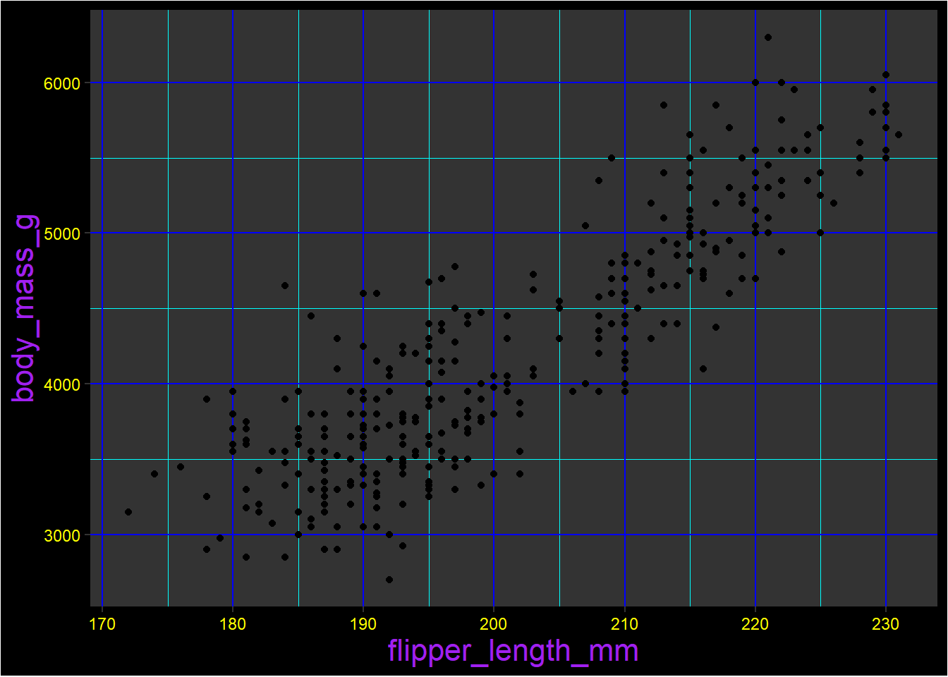
Highly customize the
theme()component (you can make it as bright / awful as you want - this is going to become a ggplot theme you can share with the world, so it’s up to you). Here’s something awful just to remind you of what this can look like:
ggplot(data = penguins, aes(x = flipper_length_mm, y = body_mass_g)) +
  geom_point() +
  theme(title = element_text(size = 16, color = "purple"),
        plot.background = element_rect(fill = "black"),
        panel.background = element_rect(fill = "gray20"),
        axis.text = element_text(color = "yellow"),
        panel.grid.major = element_line(color = "blue"),
        panel.grid.minor = element_line(color = "cyan")
  )
## Warning: Removed 2 rows containing missing values (geom_point).
- Create your own package, choose any name you want (e.g., theme_eighties)
This exercise was extracted and adapted from [link]{.ul}.
Conditionals
Challenge 1: Check records for a specific year
Download the gapminder dataset available here. This data includes years of numerous country-level indicators of health, wealth and development. Use an if() statement to print a suitable message reporting whether there are any records from 2002 in the gapminder dataset.
Can you write a function and try the same for year 2012?
Challenge 2: Thesis data
To determine if a file named thesis_data.csv exists in your working directory you can use list.files() to get a list of available files and directories.
-
Use the
%in%operator to write a conditional statement that checks ifthesis_data.csvis in this list. -
Write an
ifstatement that loads the file usingread.csv()only if the file exists. -
Add an
elseclause that prints “OMG MY THESIS DATA IS MISSING. NOOOO!!!!” if the file doesn’t exist. -
Make sure your actual thesis data is backed up.
Loops
Challenge 1: Processing multiple files
In the folder Rainfall_QLD we have multiple files with information of monthly rainfall (units are millimetres) for different stations in Queensland. We are only interested in those files ending in _Data12.csv. Write a function called analyze_all that takes a folder path and a filename pattern as its arguments and runs analyze_precip() a function that computes and plot the monthly (like the function like the you made for the monthly precipitation in Gainesville exercise) for each file whose name matches the pattern. Include in the plot the name of the station number.
The function should also generate a text file with the name “task_complete” if loop is successfully executed or “warning” otherwise.
Challenge 2: Bird communities
We have data on bird communities that we’ve collected that we need to analyse. The data has three columns, a date, a common name, and a count of the number of individuals:
2013-03-22 bluejay 5
2013-03-22 mallard 9
2013-03-21 robin 1
We want to count the total number of individuals of each species that were seen in each data file. Write two functions get_raw_data() and get_species_counts() that help you with this. Count the number of individuals of each species in a data file.
This is great for a single data file with a particular name, but we’ve been collecting data on birds from a number of different places and we’d like to conduct all of these analyses simultaneously. Write a simple for loop that loops over all of the files in the data directory that have the general form of data_*.txt, prints out the name of the data file, and then uses the functions you’ve created previously on the data file. Save this in a text file called all_species_counts.txt.
Challenge 3: Exploring correlations
For this challenge we will use a dataset (Bats_data.csv) where bats were sampled across regrowth forest in south-eastern Australia which has been thinned to reduce the density of trees.
Bats <- read.csv(file="data/Bats_data.csv", header=T, stringsAsFactors=F)
str(Bats)
Having a look at the structure of this data, we have two response variables: activity (no. of bat calls recorded in a night) and foraging (no. of bat feeding calls recorded in a night). These data were collected over a total of \(173\) survey nights and at \(47\) different sites. There are eight potential predictor variables in the data frame, one of which is a factor (Treatment.thinned), and seven of which are continuous variables (Area.thinned, Time.since.thinned, Exclusion.thinned, Distance.murray.water, Distance.creek.water, Mean.T, Mean.H).
Let’s say we are exploring our data and we would like to know how well bat activity correlates with our continuous covariates. We’d like to calculate Pearson’s correlation coefficient for activity and each of the covariates separately. Pearson’s correlation coefficient, calculated with the function cor, ranges from -1 (perfect negative correlation) to 1 (perfect positive correlation) with 0 being no correlation.
Write a code to generate a new data frame called Correlations where we can store in one column the name of the continuous covariate and its Pearson’s correlation coefficient with activity in another.
Extracted from here.
Challenge 4: Breaking a loop
Sometimes in simulations you need to know when a condition is met. Let’s suppose a population of plants follows the logistic relationship: $$N_{t+1} = r N_t \left( \frac{K-N_t}{K} \right) + N_t $$
where \(N_{t+1}\) is the population size at time \(t+1\), \(N_t\) is the population size at time \(t\), \(K\) is the carrying capacity and \(r\) is the growth rate. The Forest Service will apply an herbicide treatment when the population exceeds 30 plants per acre, but they need to know when this will happen given the model.
-
Can you determine the value? Look for some information about
?break. -
Simulate a population for a 100 year period assuming is described by a logistic function with the following parameters:
\(r = 0.15\)year$^{-1}$,\(N_0 = 6\)plants hectare$^{-1}$ and\(K = 49\). Simulate the population for 100 years and report the population size at year 89. Make a plot of the population over time.
Debugging
Challenge 1: Find the bugs
Find the bugs in buggy-granger-analysis-code-R.R and fix them. You’ll need to both read the code and use a debugger to understand what’s going on and fix the problems. Get the code cleaned up at least up to the point where the code is actually executing.
Challenge 2: get_climates()
a) Determine the bug when you run get_climates(). Hints: you can use traceback() to find where it occurs, add breakpoints / browser() calls and look at types of input
b) If you successfully found and fix the bug in get_climates(). Try running the function for a different file called “moar_planets.csv”.
What happen? Are you getting the expected values?
Debug it and see if it still runs for the previous file “planets.csv”.
This exercise was extracted from Amanda Gadrow’s great webinar Debugging techniques in RStudio.