What are we going to learn?
R is a great tool to go from importing to reporting. This afternoon, we focus on the “reporting” part.
Using R, RStudio, the R Markdown syntax and the knitr package, we can create reproducible reports that mix code and prose. If the underlying data changes, we only need to replace the original data file and “knit” the report once more, which updates all its contents in one click.
Create a new R Markdown file
We can stick to the workshop’s project, but we need to create a new R Markdown file: “File > New File > R Markdown….” We can change the title of the report, and the author as well. Let’s stick to “HTML document” as an output for now.
R Markdown and knitting
See how the document is already populated with a template? Scroll through and have a look at how it is structured. The three main elements are:
- a YAML header at the top, between the
---tags; - Markdown sections, where we can write prose, format text and add headers;
- and code chunks, in between
```where we can write R code.
But before we edit this document, let’s go straight to the “knit” button at the top of the source panel. Clicking that button will compile a document from the R Markdown file. You should see the process unfolding in the R Markdown tab, and the HTML document pop up in a separate window when it is finished.
See how the document contains a title, headers, code input and output, and explanations?
Editing the document
Let’s remove everything below our YAML header, and start writing our own report!
Markdown syntax
To add a header, we can start a line with ##: this will be a header of level 2. The number of hash symbols corresponds to the level of the header. See how the highlighting changes in the source editor?
We are going to deal with our lizard dataset, so let’s add a header and some text about the source of the data. For example:
## Lizard size measurement data

Our data comes from the [Jornada Basin Long Term Ecological Research (LTER) site](https://lter.jornada.nmsu.edu/) in New Mexico.
Notice how we used a [text](link) syntax to add a link to a website?
Challenge 1
We can also style our text by surrounding with other tags:
**for bold*for italic
Try to style your text, and add a header of level 3 for a section on “importing the data.” Knit the document to see if it works!
R code chunks
We can now add a code chunk to include some R code inside our reproducible document. To add a code chunk, click the “Insert” button at the top of the source panel, and click “R.” You can see that the language of the code chunk is defined at the top, with {r}.
Let’s import the Tidyverse, by including this code in the chunk:
library(tidyverse)
Notice that you can run your chunks of code one by one by clicking the green “play” button at the right of the chunk: you don’t have to knit the whole document every time you want to test your code.
Now, try to knit the document and see what it looks like.
Challenge 2
Inside a new chunk, add some code to import the dataset we previously prepared into an object called lizards.
lizards <- read_csv("data/lizards.csv") %>%
  mutate(date = lubridate::mdy(date))
Clicking “Knit” will automatically save your .Rmd file as well as the HTML output.
Now, we can add a chunk to show the data, by including this code in it:
lizards
## # A tibble: 1,628 × 16
##    date       scientific_name   common_name  zone  site  plot    pit spp   sex
##    <date>     <chr>             <chr>        <chr> <chr> <chr> <dbl> <chr> <chr>
##  1 1989-06-16 cnemidophorus ti… western whi… c     cali  a         4 cnti  m
##  2 1989-06-16 uta stansburiana  side-blotch… c     cali  a         8 utst  j
##  3 1989-06-16 cnemidophorus ti… western whi… c     sand  b         2 cnti  m
##  4 1989-06-16 cnemidophorus ti… western whi… c     sand  b         8 cnti  f
##  5 1989-06-16 cnemidophorus ti… western whi… c     sand  c         2 cnti  m
##  6 1989-06-16 cnemidophorus ti… western whi… g     basn  b         1 cnti  f
##  7 1989-06-16 uta stansburiana  side-blotch… g     basn  b         2 utst  f
##  8 1989-06-16 cnemidophorus te… colorado ch… g     basn  b         8 cnte  j
##  9 1989-06-16 cnemidophorus te… colorado ch… g     basn  b         9 cnte  f
## 10 1989-06-16 cnemidophorus ti… western whi… g     basn  b        10 cnti  m
## # … with 1,618 more rows, and 7 more variables: rcap <chr>, toe_num <dbl>,
## #   sv_length <dbl>, total_length <dbl>, weight <dbl>, tail <chr>, pc <dbl>
Data frames (and tibbles) don’t look particularly nice when printed as is into an R Markdown document. There are however many tools available to make a table look nice, for example knitr::kable().
Let’s try it in a new chunk:
lizards[1:5,1:4] %>% # only a small subset
  knitr::kable()
| date | scientific_name | common_name | zone |
|---|---|---|---|
| 1989-06-16 | cnemidophorus tigrisatus | western whiptail | c |
| 1989-06-16 | uta stansburiana | side-blotched lizard | c |
| 1989-06-16 | cnemidophorus tigrisatus | western whiptail | c |
| 1989-06-16 | cnemidophorus tigrisatus | western whiptail | c |
| 1989-06-16 | cnemidophorus tigrisatus | western whiptail | c |
The R Markdown cheatsheet lists other table tools that should cover most needs.
Working directory
Note that the working directory for an R Markdown document will be the .Rmd file’s location by default (and not necessarily the working directory of the R project your are in). That is why it is a good idea to save your R Markdown file at the top of your R Project directory if you want consistency between your scripts and your R Markdown file.
When we import a data file, we have to remember to use a path relative to the location of the .Rmd file.
You can change the default behaviour by using the Knit dropdown menu and choosing an option in “Knit directory.”
Chunk options
Notice how our two first chunks show some messages as an output? We might want to remove that if it is not important and we don’t want to include it in the report. At the top of your chunk, you can modify the options like so:
The code will be executed and the output (if there is any) will be shown, but the messages won’t!
There are many options to choose from, depending on what you want to do and show with your chunk of code. For example, to hide both messages and warnings, and only show the output of the code (without showing the underlying code), you can use these options, separated by commas:
It also is a good idea to label your chunks, especially in longer documents, so you can spot issues more easily. It won’t be shown in the report, but will be used in the R Markdown console and can be used to navigate your script (with the dropdown menu at the bottom of the source panel). For example, for our first chunk:
library(tidyverse)
It is also possible to include a chunk at the top of your document, that will detail the default options you want to use for all you chunks. That is particularly useful if you want to define a default size for all your figures, for example.
Here is an example of a chunk you might use to change default options:
```{r setup, include=FALSE}
knitr::opts_chunk$set(echo = TRUE, message = FALSE, warning = FALSE)
```
That would make sure that, by default:
- The code is shown, but
- the messages and warnings are hidden.
Errors when knitting
It should be straight forward to find where an issue comes from when knitting a report does not work.
Challenge 3
Try changing a chunk code so the code is not valid. What can you see in the R Markdown console?
Double-click on the error message to jump the problem.
Inline code
We can also include code that will be executed inside Markdown text. For example, you can write the following sentence:
The dataset contains observations spanning the period
`r min(lizards$date)`to`r max(lizards$date)`. It focuses on`r length(unique(lizards$scientific_name))`species and the heaviest specimen is`r max(lizards$weight)`g.
We can also use this feature to auto-update the date of your report every time it is knitted. Replace the date line in the YAML header with this one:
date: "`r Sys.Date()`"
Now, try knitting the report again.
Visualisation
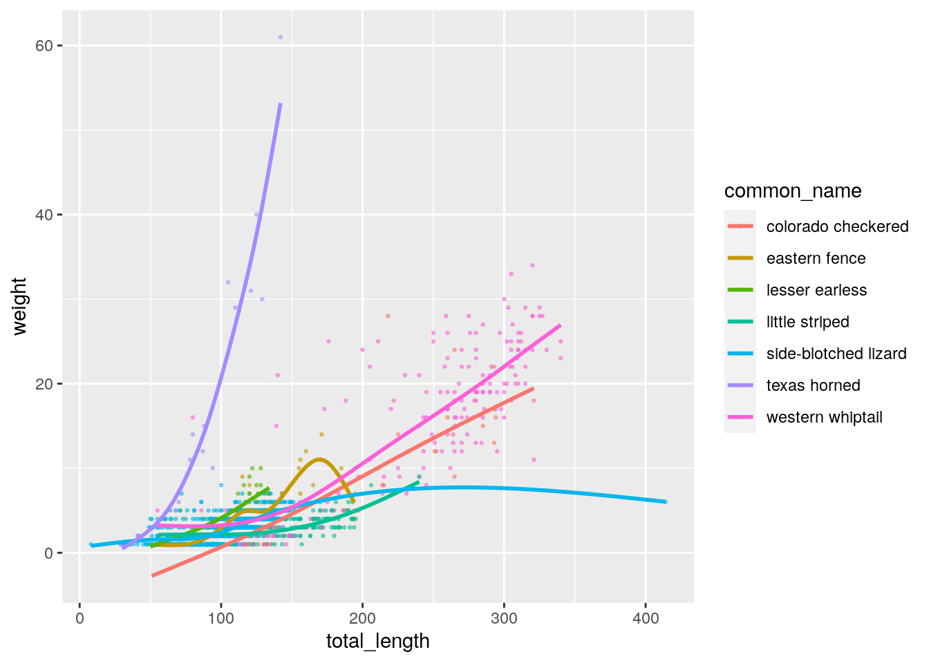
Let’s include a visualisation using, for example, ggplot2:
p <- ggplot(lizards, aes(x = total_length, y = weight, colour = common_name)) +
  geom_point(alpha = 0.5, size = 0.5) +
  geom_smooth(se = FALSE)
p
## `geom_smooth()` using method = 'gam' and formula 'y ~ s(x, bs = "cs")'
If you want to hide the code that created an output, like for this plot, you can add the option
echo=FALSEto it.
The Texas Horned lizard doesn’t vary much in length but does a lot more in weight.
Images
We now want to illustrate our report with this Public Domain image of a Texas Horned lizard.
Inserting an image in Markdown requires a syntax similar to hyperlinks: 
You can add this to your document:


When R Markdown syntax becomes cumbersome (for example when creating a static table from scratch), one of RStudio’s newest features becomes very handy: the Visual Markdown Editor. Click on the compass icon at the top right of the source panel and try editing the document with the toolbar.
Interactive visualisations
Finally, let’s create an interactive version of our plot. The plotly package makes it trivial to convert a static ggplot2 visualisation to an interactive version:
library(plotly)
##
## Attaching package: 'plotly'

## The following object is masked from 'package:ggplot2':
##
##     last_plot

## The following object is masked from 'package:stats':
##
##     filter

## The following object is masked from 'package:graphics':
##
##     layout
ggplotly(p)
## `geom_smooth()` using method = 'gam' and formula 'y ~ s(x, bs = "cs")'
This will work in a HTML document, but will most likely fail in other output formats.
If you want to change the size of your visualisations, you can tweak the width and height with chunk options. However, you make that consistent for all your figures, by using an extra default option in the setup chunk (the one that contains the {r setup, include=FALSE} header, at the top of the document). For example:
knitr::opts_chunk$set(fig.width = 8)
Being respectful of APIs
R is a great tool to acquire data from various databases. For example, to find observations of the genus Phrynosoma in New Mexico, we could use the rinat package and download data from iNaturalist.
However, given that we keep modifying our report and that the code is run every time we compile the document, it might be a good idea to not put too much load on the data provider, and store that code in a separate script. (It will also make compiling quicker.)
Create a new script called get_inat_data.R, and include this code in it:
# get observations of horned lizards in New Mexico
library(rinat)
phryno <- get_inat_obs(taxon_name = "Phrynosoma",
                      place_id = 9,
                      quality = "research",
                      geo = TRUE,
                      maxresults = 300)
# convert to a spatial vector object
library(sf)
phryno <- st_as_sf(phryno, coords = c("longitude", "latitude"))
# export
st_write(phryno, "data/phryno.geojson")
When run, the script:
- Gets the relevant data from the iNaturalist API
- Converts the data frame to an sf object
- Exports it as a geojson file
This code only needs to be run once (or anytime the data needs updating).
We can then include in the R Markdown report the necessary code to import and visualise the data. We need to read the geojson file, and we can then visualise it with tmap:
# import the prepared data
library(sf)
phryno <- st_read("data/phryno.geojson")
# visualise on interactive map
library(tmap)
tmap_mode("view")
tm_shape(phryno) +
  tm_dots(col = "common_name",
          popup.vars = c("common_name", "scientific_name", "place_guess"))
Update the report
If you have an updated version of the dataset, the only thing you need to do to update the whole report is point the data import code to the new file, at the top of our document.
Knitting again will update all the objects and visualisations for us! This is the power of reproducible reports in R.
With reproducible reports, you can potentially structure and write (most of) a report even before you have your research project’s final dataset. (Well, at least the data analysis part, maybe not so much the conclusions!)
Output formats
HTML documents
The benefits of using HTML documents are multiple:
- figures won’t break the flow of the document by jumping to the next page and leaving a large blank space;
- you can include interactive visualisations making use of the latest HTML features;
- they can be directly integrated into a website.
However, other output formats are available. Here are some examples:
pdf_documentfor a non-editable, widespread, portable formatword_documentandodt_documentto open and edit with Microsoft Word and LibreOffice Writermd_documentfor a Markdown file that can easily be published on GitHub or GitLab- and more, including for creating slides.
Knitting to PDF
In some cases, you might be required to share your report as a PDF. Knitting your document to PDF can generate very professional-looking reports, but it will require having extra software on your computer.
You can install the necessary LaTeX packages with an R package called TinyTeX, which is a great alternative to very big LaTeX distributions that can be several gigabytes-big.
install.packages("tinytex")
tinytex::install_tinytex()
After this, try to change your YAML header’s output value to pdf_document and knit it. But remember that you might have to “turn off” certain HTML-only elements like the interactive visualisations (for example by using eval=FALSE in the chunks).
Useful links
Related to R Markdown and knitr:
- R Markdown Cookbook, by Yihui Xie and Christophe Dervieux
- Official R Markdown website by RStudio
- R Markdown cheatsheet